Matrix Math on a Commodore 64
By Michael Doornbos
- 15 minutes read - 3033 wordsThe fly-hash port from a few weeks back ended with a sparse matrix multiply, and I more or less waved a hand at what that meant and kept going. The SID-as-reservoir-computer leans on a linear regression to read out its results, which is also matrix algebra all the way down. Both of them skip over the actual math, so here’s the clean reference I should have written first. Python first, because that’s where you’d write this in 2026, and then on a Commodore 64, because of course we will. The 2 by 2 in the photo up top, I worked out by hand first, on graph paper with a slide rule, just to have something to check the machines against.
What is linear algebra
Linear algebra is the math of linear relationships. “Linear” is the word doing the work: scaling an input scales the output by the same factor, and adding two inputs adds their outputs. y = 3x is linear, double the x and the y doubles right along with it. So is z = 2x + 5y. Put an x² or a sine in there and it stops being linear, and you’ve wandered off into a harder branch of math.
That sounds like a narrow corner to build a whole field on, but linear relationships are everywhere, and plenty of things that aren’t quite linear are close enough that treating them as linear gets you a useful answer.
A few everyday ones:
- Scaling a recipe. Cook for twice as many people and every ingredient doubles. The output tracks the input in lockstep.
- The total at the register. Each item’s price times its quantity, all added up. Bump any one quantity and the total moves by the same proportion.
- Mixing. Blend a 10% solution with a 40% one and the strength of what you end up with is a straight average, weighted by how much of each you pour in.
Stack a pile of these relationships together and you need a way to write them all down and work on them at once. That’s what matrices are for, which is why a field named after straight lines spends most of its time pushing grids of numbers around.
What is a matrix
A matrix is a grid of numbers, rows down the side and columns across the top, with a value sitting in each cell. The word makes it sound bigger than it is. A spreadsheet is a matrix. So is the screen on a Commodore 64, if you’re willing to count the character codes.
We talk about a matrix’s shape as rows by columns, in that order. The grid below is a 2 by 3, two rows and three columns:
[ 1  2  3 ]
[ 4  5  6 ]
Some shapes get their own names. A matrix with a single column is a column vector. With a single row, a row vector. One with the same number of rows as columns is square. A 1 by 1 is just a number, which mathematicians insist on calling a scalar so it sounds like it’s earning its keep.
When you index into a matrix, the convention is row first, then column, so the 6 above is at row 2, column 3. Math books index from 1, Python indexes from 0, and Commodore BASIC also indexes from 0, but everybody quietly pretends it doesn’t. We’ll come back to that when we get to BASIC.
What are they good for
Once you start looking, they’re everywhere. Anything naturally laid out in two dimensions is already a matrix, even if nobody used the word.
They’re how you solve systems of linear equations. A pair like 2x + 3y = 7 and 4x - y = 1 is easy on paper, but two thousand of them need a different approach, so you stack the coefficients into a matrix and let linear algebra do the work.
The other place they show up is in transformations. Rotations, scales, projections. Every game with 3D graphics is doing a pile of matrix multiplications per frame. Neural networks are stacks of matrix multiplications with a non-linear function sprinkled in between. The fly-hash random projection that started this rabbit hole is a single matrix multiplication with a sparse weight matrix.
The large language models everyone’s been talking about are the same idea taken to a ridiculous scale. When one reads your prompt and writes back, nearly all of the real work is matrix multiplication. Each chunk of text becomes a list of numbers, a vector, and the model pushes those vectors through layer after layer of weight matrices. That includes the attention step, where it works out how much each earlier word should pull on the next one, which is itself a matrix multiplication. It’s all dot products, the same operation as the 2 by 2 further down, except the matrices hold billions of numbers and a graphics card grinds through them in parallel. Producing one token, roughly a word, takes millions of multiply-and-add steps. The arithmetic is exactly what we’re about to run on a Commodore 64. Only the size and the speed change.
The reason a graphics card is the right tool here is half an accident of history. A matrix multiply breaks down into thousands of little dot products that don’t depend on each other, so you can hand each one to a different worker and run them all at the same time. A regular processor has a handful of fast cores and grinds through the list more or less in order. A GPU has thousands of slower ones and takes the whole batch at once. It ended up that way because drawing 3D graphics is the same kind of work, the same transform applied to every corner of every shape and every pixel on its own, so the chip built to spin triangles in games turned out to be exactly what a neural network wanted.
The operations
There are four operations worth knowing up front: addition, subtraction, scalar multiplication, and matrix multiplication. Plus transpose, which is more of a rearrangement than an operation, and division, which I’ll get to at the end when I admit it’s a small lie.
Addition and subtraction
To add two matrices, add the corresponding entries. The shapes have to be identical, otherwise there’s nothing to match.
[ 1  2 ]   [ 5  6 ]   [  6   8 ]
[ 3  4 ] + [ 7  8 ] = [ 10  12 ]
Subtraction works the same way with a minus sign in the middle:
[ 1  2 ]   [ 5  6 ]   [ -4  -4 ]
[ 3  4 ] - [ 7  8 ] = [ -4  -4 ]
Scalar multiplication
Multiply every cell by the same number. That’s it.
    [ 1  2 ]   [ 3   6 ]
3 * [ 3  4 ] = [ 9  12 ]
You use this any time you want to rescale all the values in a matrix at once, whether that’s for a unit conversion or to apply a learning rate to a neural network’s weights.
Matrix multiplication
This is the operation that earns its keep, and it’s also the one that confuses everybody the first time, because it doesn’t behave the way addition does. The rule is that the inner dimensions have to match. If A is m by n and B is n by p, then A times B is an m by p matrix, and the shared n collapses out of the result. Each cell of that result is a dot product: take a row from A, take a column from B, multiply matching elements, and add them up.
[ 1  2 ]   [ 5  6 ]   [ 1*5+2*7   1*6+2*8 ]   [ 19  22 ]
[ 3  4 ] * [ 7  8 ] = [ 3*5+4*7   3*6+4*8 ] = [ 43  50 ]
The order matters here. A*B and B*A are usually different, and sometimes one of them isn’t even defined because the shapes don’t line up. And the matrices don’t have to be square, as long as the inner dimensions agree. A 2 by 3 multiplied by a 3 by 4 gives you a 2 by 4.
Transpose
Flip the matrix across its diagonal, so rows become columns and vice versa. The transpose of an m by n matrix is n by m.
[ 1  2  3 ] T   [ 1  4 ]
[ 4  5  6 ]  =  [ 2  5 ]
                [ 3  6 ]
It shows up all over the place once you start doing real work, especially in the formulas for linear regression and PCA. PCA is principal component analysis, a way of finding the few directions in which your data varies the most and throwing away the rest, so a table with hundreds of columns can be squeezed down to the handful that actually carry the information.
Division (kind of)
There is no such thing as matrix division. The nearest equivalent is multiplication by an inverse, the matrix A to the minus one, such that A * A^-1 = I, where I is the identity matrix with ones down the diagonal and zeros everywhere else. Not every matrix has an inverse, and computing one is its own algorithm with several flavors.
Some libraries offer “element-wise division” as a convenience, in which each cell of A is divided by the corresponding cell of B. That’s a useful shortcut for operations like normalization, but it isn’t matrix division in the linear algebra sense. It’s just doing the same thing to each pair of numbers, the way addition and subtraction work.
Python first
I’m going to do all of this in plain nested lists, no numpy yet, so the gears stay visible. Numpy shows up in a moment.
A matrix is a list of rows, where each row is a list of numbers. A 2 by 3 looks like this:
A = [[1, 2, 3],
     [4, 5, 6]]

B = [[5, 6],
     [7, 8],
     [9, 10]]
A small helper for printing them so we can read what’s going on:
def show(M):
    for row in M:
        print(" ".join(f"{x:4}" for x in row))
    print()
Addition walks every cell with a list comprehension, no surprises:
def add(A, B):
    rows, cols = len(A), len(A[0])
    return [[A[i][j] + B[i][j]
             for j in range(cols)]
            for i in range(rows)]
Subtraction is identical with a minus sign. Scalar multiply is even simpler:
def scale(k, A):
    return [[k * x for x in row] for row in A]
Matrix multiply is the triple-nested loop you’ve seen in every linear-algebra textbook. The outer two loops walk the cells of the result, and the inner loop computes the dot product for that one cell:
def matmul(A, B):
    m, n  = len(A), len(A[0])
    n2, p = len(B), len(B[0])
    assert n == n2, "inner dimensions must match"

    C = [[0] * p for _ in range(m)]
    for i in range(m):
        for j in range(p):
            s = 0
            for k in range(n):
                s += A[i][k] * B[k][j]
            C[i][j] = s
    return C
Transpose is one line if you know that zip(*A) does most of the work for you:
def transpose(A):
    return [list(row) for row in zip(*A)]
Putting it all together:
A = [[1, 2], [3, 4]]
B = [[5, 6], [7, 8]]

show(add(A, B))      # element-wise sum
show(scale(3, A))    # scalar times A
show(matmul(A, B))   # the real multiply
show(transpose(A))   # rows become columns
Output:
   6    8
  10   12

   3    6
   9   12

  19   22
  43   50

   1    3
   2    4
That’s a complete introductory matrix library in around thirty lines of Python. Almost every fancier matrix routine builds on these primitives.
Where numpy fits
The version above is fine for understanding what matrix multiplication is. For doing matrix work on anything bigger than a textbook example, you reach for numpy instead. The interface is similar enough that switching is painless, and the speed is in another league.
import numpy as np

A = np.array([[1, 2], [3, 4]])
B = np.array([[5, 6], [7, 8]])

A + B           # element-wise sum
3 * A           # scalar multiply
A @ B           # matrix multiply
A.T             # transpose
The @ operator means matrix multiplication. The * operator is element-wise: every cell of A is multiplied by the matching cell of B, with no dot-product collapse. They’re easy to mix up the first time, and the difference matters.
The reason numpy matters is speed. A 1000-by-1000 matrix multiplication with the nested-loop code above runs in about 30 seconds on a modern laptop. Numpy does the same work in roughly 15 milliseconds, three orders of magnitude faster.
The Commodore 64 doesn’t have a numpy.
Commodore BASIC
BASIC’s turn, in a language designed back when “object-oriented” meant “I’m pointing at it”.
DIM A(3,3) allocates a 4-by-4 grid, since BASIC includes both bounds. I’m using indices 1 through N and ignoring row 0 and column 0, the way a math book would. Costs a few bytes, saves the whole article from off-by-one.
Here’s the program. It prints both source matrices side by side at the top so the inputs are right there next to the results, then runs each operation.
10 REM MATRIX BASICS ON A C64
20 PRINT CHR$(147);CHR$(5)
30 DIM A(2,2),B(2,2),C(2,2)
40 A(1,1)=1:A(1,2)=2
50 A(2,1)=3:A(2,2)=4
60 B(1,1)=5:B(1,2)=6
70 B(2,1)=7:B(2,2)=8
80 PRINT "MATRIX A";TAB(15);"MATRIX B"
85 FOR I=1 TO 2
86 FOR J=1 TO 2:PRINT A(I,J);:NEXT J
87 PRINT TAB(15);
88 FOR J=1 TO 2:PRINT B(I,J);:NEXT J
89 PRINT:NEXT I
90 PRINT
100 PRINT "A + B"
110 FOR I=1 TO 2:FOR J=1 TO 2
120 C(I,J)=A(I,J)+B(I,J):NEXT J,I
130 GOSUB 1000:PRINT
200 PRINT "3 * A"
210 FOR I=1 TO 2:FOR J=1 TO 2
220 C(I,J)=3*A(I,J):NEXT J,I
230 GOSUB 1000:PRINT
300 PRINT "A * B"
310 FOR I=1 TO 2:FOR J=1 TO 2
320 S=0
330 FOR K=1 TO 2:S=S+A(I,K)*B(K,J):NEXT K
340 C(I,J)=S:NEXT J,I
350 GOSUB 1000:PRINT
400 PRINT "A TRANSPOSED"
410 FOR I=1 TO 2:FOR J=1 TO 2
420 C(J,I)=A(I,J):NEXT J,I
430 GOSUB 1000
500 END
1000 REM PRINT MATRIX C
1010 FOR I=1 TO 2
1020 FOR J=1 TO 2
1030 PRINT C(I,J);
1040 NEXT J:PRINT
1050 NEXT I
1060 RETURN
Running it gives you this:
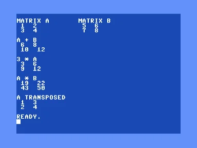
Inputs across the top so you can check the work yourself, results underneath. A times B lands on the same 19, 22, 43, 50 we ground out by hand on the graph paper.
Slowly, of course, which is half the point.
Bigger matrices
The 2 by 2 lands instantly. Push it up to 10 by 10, a thousand multiplications and a thousand additions, and BASIC starts to drag.
Same algorithm, scaled up:
10 REM 10X10 MATMUL TIMING
20 PRINT CHR$(147);CHR$(5)
30 N=10
40 DIM A(N,N),B(N,N),C(N,N)
50 FOR I=1 TO N:FOR J=1 TO N:A(I,J)=I:B(I,J)=J:NEXT J,I
60 PRINT N;"X";N;"MATMUL IN BASIC"
70 PRINT "TIMING..."
80 TI$="000000"
90 FOR I=1 TO N:FOR J=1 TO N
100 S=0
110 FOR K=1 TO N:S=S+A(I,K)*B(K,J):NEXT K
120 C(I,J)=S:NEXT J,I
130 T=TI/60
140 PRINT
150 PRINT "ELAPSED:";T;"SEC"
160 PRINT
170 PRINT "C(1,1) =";C(1,1)
180 PRINT "C(5,5) =";C(5,5)
190 PRINT "C(10,10)=";C(10,10)
The pattern A(I,J) = I, B(I,J) = J has a closed form C(I,J) = N*I*J, so the three sample cells should be 10, 250, and 1000.
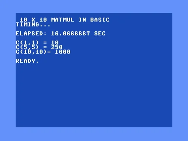
A thousand multiplies in BASIC, 16.07 seconds on the jiffy clock. The three spot-checks come out to 10, 250, and 1000, right where the closed form says they should.
Sixteen seconds for a thousand multiplications. Not bad.
The same multiply in assembly
Same algorithm in 6502, calling the BASIC ROM’s float routines directly. The four we need are:
$bba2MOVFM — load FAC from memory$ba28FMULTT — multiply FAC by a value in memory$b867FADDT — add a value in memory to FAC$bbd4MOVMF — store FAC to memory
A matmul cell is exactly the dot-product loop wrapped around those four calls. For each k from 0 to N-1, load A[i,k] into FAC, multiply by B[k,j], add the running sum from a five-byte scratch, and store the new sum back. After the loop, FAC still holds the final cell value, ready to write into C[i,j]:
; inner k loop: sum += a[i,k] * b[k,j]
mk      jsr addraik     ; ptr = address of a[i,k]
        lda ptr
        ldy ptr+1
        jsr movfm       ; fac = a[i,k]
        jsr addrbkj     ; ptr = address of b[k,j]
        lda ptr
        ldy ptr+1
        jsr fmultt      ; fac = fac * b[k,j]
        lda #<sumf
        ldy #>sumf
        jsr faddt       ; fac = fac + sum
        ldx #<sumf
        ldy #>sumf
        jsr movmf       ; sum = fac
        inc k
        lda k
        cmp #n
        beq donek
        jmp mk
donek
The fiddly part is the addressing. Each matrix is a flat array of 5-byte floats row by row, so A[i,k] sits at base + i*50 + k*5. Two precomputed tables handle that: row offset i*50 (split into low and high bytes since some overflow), and column offset j*5 (always single-byte for a 10x10). Any cell address is base + row offset + column offset.
GIVAYF at $b391 is documented in several published references as A=low, Y=high. The standard 901226-01 BASIC ROM does the opposite: A is the high byte, Y is the low byte. Get them backward on small values, and every result comes out exactly 256 times too large.
Running it:
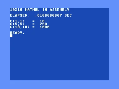
The same thousand multiplies through the ROM’s float routines, done in a single jiffy. Same three answers, about 960 times quicker than BASIC.
About 960 times faster.
How they compare
Multiplies per second for each:
| Implementation | Multiplies per second |
|---|---|
| C64 BASIC V2 | 62 |
| C64 6502 + BASIC ROM floats | 60,000 |
| CPython 3 triple loop | 33 million |
| Numpy, single core | 76 billion |
A factor of about a billion from top to bottom, on hardware separated by forty years.
That four-step MOVFM / FMULTT / FADDT / MOVMF pattern is good for almost any float work on the C64. Once you have it, the rest of linear algebra opens up. Solving a system of equations, the forward pass of a small neural network, the random projection that drives the fly-hash port that started this thread. Matrices look dull on paper. They get interesting when you can run them on something the size of a breadbox. And it’s even better if it’s Commodore brown.