Biological Processing Units and a Commodore 64
A scientist at Johns Hopkins named Joshua Vogelstein and his lab did something unusual in 2025. They took a map of a fruit fly larva’s brain, every single neuron and every wire between them (about 3,000 cells and 65,000 connections), and used it as the skeleton of an artificial intelligence program.
Most AI you hear about today uses a structure called a transformer. Transformers do a lot, but they were built from scratch by humans. Nobody fully understands why their internal wiring works, and they burn a staggering amount of electricity. A single query to one of today’s big models uses more energy than a fruit fly’s entire brain uses in a day.
Vogelstein’s idea was simple. Evolution has already designed working brains over hundreds of millions of years. A fruit fly’s brain is tiny compared to ours, but it flies, navigates, remembers smells, learns, and makes decisions on about 6 milliwatt-hours per day. Why not use that design as a starting point for AI?
You don’t try to simulate a living fly brain. You take the wiring diagram (scientists call it a connectome), freeze it as the backbone of a computer program, and only train the input and output layers. (“Layers” is the word AI people use for the horizontal slabs of a neural network. A network is a stack of layers, each one doing some math on its input and handing the result up to the next.) The brain in the middle stays exactly as the fly has it. The program learns by figuring out how to feed data into the fly brain and read the answer back out.
Vogelstein called this a Biological Processing Unit, or BPU. On simple tasks like recognizing handwritten digits, it did about as well as a standard AI with many more moving parts. On the ChessBench benchmark, a 2-million-parameter BPU beat a parameter-matched transformer head to head (74% vs 67% puzzle accuracy), and with minimax search added at inference, reached 91.7%, exceeding even a 9-million-parameter transformer baseline. ChessBench is a standard AI test: feed the model millions of real chess positions and score how often it picks the move a strong chess engine would play. Even more striking, a 233,000-parameter BPU trained on only 10,000 games was roughly 10 times as accurate on puzzles as any transformer the authors tested at that small-data budget, including a 270-million-parameter baseline. The rule of thumb in modern AI is “more parameters win.” This result says the fly’s wiring is pulling its weight. A smaller network shaped like a real brain can beat a bigger one built from scratch.
Practically, that means the same job runs on a smaller computer, on less electricity, from a smaller training budget. Training a frontier-scale transformer is a data-center job costing millions of dollars and weeks of racks of GPUs. A BPU that holds its own at a fraction of the size might train on a single workstation in a few hours, then run later on a drone, a wearable, or a cheap microcontroller. The whole exercise is about closing the gap between “AI the labs demo in a paper” and “AI you can actually ship in a product.”
How This Is Different From an LLM
If you have been paying any attention to AI in the last few years, everything you hear about is a large language model, or LLM for short. The handful of top-tier ones are usually called the frontier models — as of 2026, the six that matter commercially are ChatGPT (OpenAI), Claude (Anthropic), Gemini (Google), Llama (Meta), Grok (xAI), and DeepSeek’s R series. They are all transformers, running hundreds of billions of parameters on racks of GPUs, and each one cost tens to hundreds of millions of dollars to train. A BPU is a very different animal, and the frontier-model mental model does not transfer.
A frontier LLM is a blank slate. Hundreds of billions of parameters (every tunable number inside the network: a neural net is a huge stack of multiplications and additions, and every one of those numbers being multiplied or added is a parameter the training process adjusts), all initially random. You train them by forcing the model to predict the next word on the internet, trillions of times, on racks of GPUs for weeks. After that, the knowledge sits smeared across the weights in ways nobody fully understands.
The BPU is almost the opposite. 3,016 neurons wired as a real fruit fly larva wired them, all frozen. The only weights you train are the input encoder and the output decoder, usually a few hundred thousand parameters. You can do the whole training run on a laptop in a few hours.
That is a factor of roughly 10 million in size and 10 billion in training cost. And the fly whose brain is the inspiration for the middle does a functional animal’s worth of work on that budget, not a lab curiosity’s worth.
The philosophical split is interesting. LLMs bet that if you give a blank structure enough data, it will discover everything it needs to know from scratch. That bet has worked better than anyone predicted. BPUs bet that evolution already solved a version of the problem, and rather than rediscover the answer with gradient descent (the training procedure that takes a trillion tiny nudges to a random set of weights until they produce the right outputs) on the open web, you can inherit the structure for free and just teach the edges.
The first bet is winning commercially. The second bet is interesting because it is orders of magnitude cheaper, burns orders of magnitude less electricity, and at least partly, you can look at it and explain why it works. LLMs are generalists. Ask one for a sonnet, a debugged function, or a summary of your inbox, and it will have a reasonable go at all three. A BPU is not a chatbot and never will be. It is a pattern recognizer that happens to use biology as its substrate. For anything that has to run somewhere you cannot drag a data center along (defense, wearables, satellites, anything offline-first), that narrow scope is the point. The industry word for this category is “edge computing.”
Why I’m Building This
I want to build this. Not just read the paper, actually run it on commodity platforms, because the interesting things in a paper like this live in the details that the paper does not tell you. But I want to understand what I am building before I build it. So I started with an earlier paper in the same research tradition.
The Paper That Started It
Before Vogelstein’s 2025 paper, there was a 2017 paper in Science by Sanjoy Dasgupta, Charles Stevens, and Saket Navlakha. They took a much smaller slice of the fly brain, the part that processes smell, and asked a question that is weird for a biologist and familiar for a computer scientist: What is this circuit actually computing?
The fly has about 50 types of smell receptors. Those feed into a set of roughly 2,000 neurons called Kenyon cells in a structure called the mushroom body. Each Kenyon cell samples a small, random handful of the 50 input channels from the smell receptors, maybe six. When a smell arrives, each Kenyon cell sums its six inputs. Then an inhibitory neuron (a neuron whose job is to shut other neurons off rather than make them fire more) called APL reaches across all 2,000 Kenyon cells and silences everyone except the top 5% that got the biggest sums.
What’s left is a sparse binary fingerprint. Out of 2,000 Kenyon cells, about 100 are active. That fingerprint is what the fly remembers. Two similar smells produce fingerprints that overlap a lot. Two different smells barely overlap at all.
Dasgupta and coauthors noticed that this is an exact match for a computer science tool called locality-sensitive hashing. Classical LSH takes a high-dimensional vector and produces a short binary hash such that nearby vectors get similar hashes. You use it to find “things like this one” in a big database without comparing against every entry. Reverse image search uses it. Plagiarism detectors use it. Document deduplication uses it.
The fly got there first, apparently by the late Cambrian period.
The 2017 paper’s result is that the fly’s version, what I’ll call the fly-hash, is not just as good as classical LSH. On standard benchmarks, it’s better, especially when you are allowed only a few hash bits per item. This is an earlier paper in the same research tradition that produced the 2025 BPU paper. Same fly, bigger connectome, same idea of letting biology do the hard part.
If I can reproduce the 2017 result, I will understand the 2025 result a lot better when I get there.
How the Fly-Hash Works, in Plain English
Here is the whole algorithm. I will write it out once in English and once in about fifteen lines of Python.
- You have an input vector. (A vector is just a list of numbers. The dimension is how long the list is.) For the fly, that’s 50 smell-receptor activities, so a 50-dimensional vector. For MNIST (the standard “hello world” dataset of machine learning: 70,000 handwritten digits, 28 by 28 pixels each), it’s a 784-pixel digit unrolled into one row, so a 784-dimensional vector.
- You have a big random sparse projection. Make a table of “Kenyon cells.” Each cell picks a few input dimensions at random and just adds them up. That gives you a much longer vector of activations.
- Winner-take-all. Keep only the positions with the biggest activations. Set everything else to zero. The paper uses the top 5%, so if you had 2,000 Kenyon cells you keep 100.
- The result is a sparse binary vector. That is the hash.
Explaining this at a coffee shop
Three blue dots on the left light up — those are smells hitting the fly’s nose right now. Six gold lines fan out to a single circle in the middle: that is the one Kenyon cell that happened to be watching all three of those receptors, so it wins the competition. The red bar that slides in is the APL neuron, silencing every Kenyon cell except the winner. The winner’s slot at the bottom row goes black. That row, mostly empty with one filled square, is the fly’s answer to “what is this smell?” A similar smell lights mostly the same slots. A different smell lights different ones. The similarity surviving through the hash is the whole point of the algorithm.
Two things matter here:
- The wiring is random and never changes. When each Kenyon cell is “born” in the fly, it chooses which six receptors to monitor by coin flip. That choice stays fixed for the rest of the fly’s life. No learning, no tuning, no adjustment. This is the opposite of how modern AI works: in a transformer, every single number inside the network gets nudged billions of times during training until the whole thing produces useful outputs. The fly gets its wiring for free from nature and just uses it.
- The first step makes the representation bigger, not smaller. If you’ve heard the word “hash” in programming (MD5, SHA1, Python’s
hash()), you probably think “take a big file and squash it into a tiny fingerprint.” The fly does the reverse. It takes 50 receptor readings, blows them up into 2,000 Kenyon-cell sums, and then throws away all but the loudest 5%. What comes out is a long, mostly-empty vector instead of a short, crammed one. That apparent waste is exactly what makes similar smells produce overlapping tags: a small change in the input shifts which cells are loudest slightly, rather than scrambling the whole fingerprint the way a classical hash would.
Here it is in Python, ignoring any optimization:
import random

def build_projection(n_input=50, n_kenyon=500, samples=6, seed=42):
    rng = random.Random(seed)
    return [sorted(rng.sample(range(n_input), samples)) for _ in range(n_kenyon)]

def fly_hash(input_vec, projection, wta_percent=5):
    # 1. sparse random projection: each Kenyon cell sums a few inputs
    activations = [sum(input_vec[i] for i in cell) for cell in projection]
    # 2. winner-take-all: keep the top wta_percent
    n = len(activations)
    k = max(1, n * wta_percent // 100)
    top = sorted(range(n), key=lambda i: (-activations[i], i))[:k]
    # 3. sparse binary output
    tag = [0] * n
    for i in top:
        tag[i] = 1
    return tag
That’s it. No neural network library, no GPU, no training. Fifteen lines of pure stdlib Python implements the core idea of the 2017 paper and most of the 2025 paper too.
Does It Actually Act Like a Hash?
It’s worth pausing on the word “hash.” If you come from programming, “hash” probably means MD5, SHA, or Python’s built-in hash(). Those are designed to scramble (sorta): flip one bit of input, and the output looks completely different. That is what makes them useful for checking whether a file was tampered with, or for distributing keys into a dictionary.
The fly-hash is a different kind of hash. It is locality-sensitive: similar inputs produce similar outputs. You do not use it to check whether two photos are byte-for-byte identical. You use it to find photos that are kind of like this one. Classical hash answers “Is this the same?” Locality-sensitive hash answers “which of these is the closest match?”.
A locality-sensitive hash is only useful if that property actually holds. So I built a tiny test: 20 black-and-white pictures on a 5-row by 10-column grid (fifty cells total, which conveniently matches the fly’s 50 smell channels). I arranged them in 10 pairs. Within each pair, the two images are small variations of each other (shift one pixel, add a stub, that kind of thing). Across pairs, the images are genuinely different shapes.
plus_small:        plus_wide:
..........         ..........
....##....         ....##....
..######..         .########.
....##....         ....##....
..........         ..........
The full set of twenty:
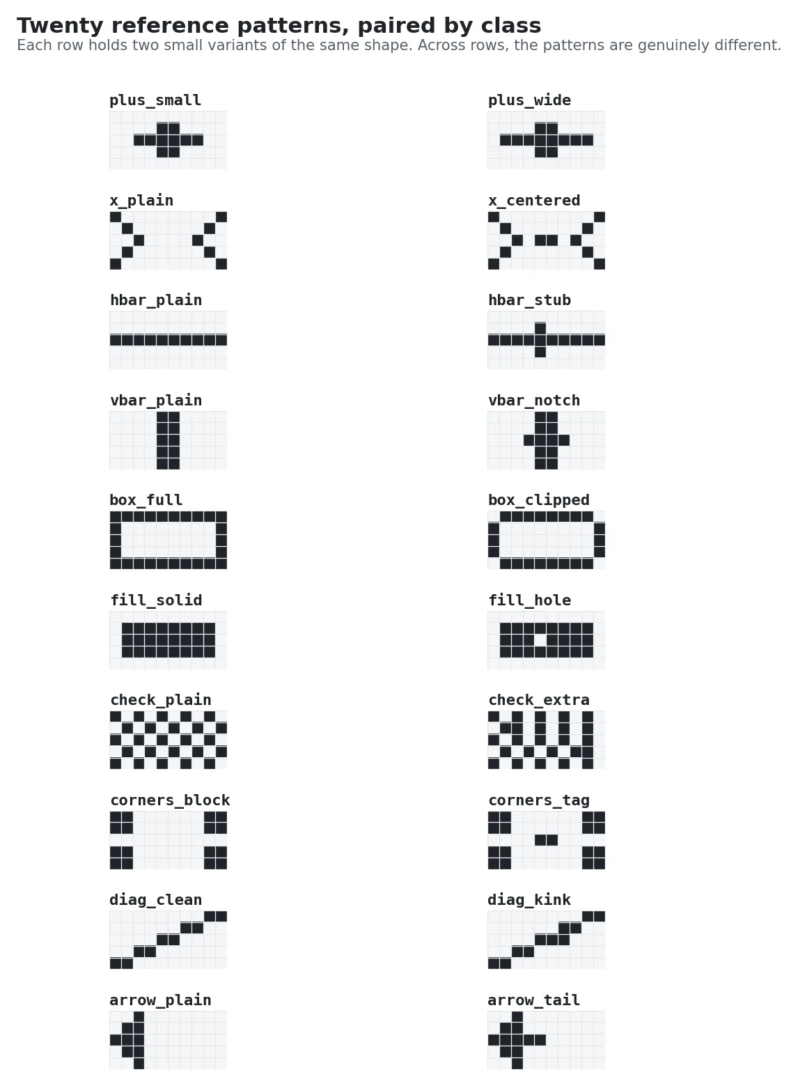
All twenty reference patterns. Each row is two class pairs; within a pair, the two patterns are small variations of each other (shift, stub, one-cell flip). Across classes, the patterns are genuinely different shapes.
If the hash works, plus_small and plus_wide should produce overlapping hashes. And neither should overlap much with, say, a checkerboard pattern.
What does “overlap” mean here? Each hash is a list of 25 winning cells (out of 500 total). The overlap between two hashes is the number of winners they share: the same cell appears in the winner lists of both. So:
- 25 out of 25 means identical hashes (every winner is shared).
- 0 out of 25 means the hashes share no cells at all.
- Random baseline: if you picked 25 winners out of 500 cells at random for each hash independently, pure chance gives you about 25 × (25/500) = 1.25 shared winners on average. Anything well above 1 is an actual signal; anything near 1 is noise.
Higher overlap = more similar. That is the signal we are looking for on within-class pairs.
Here are all ten class pairs I ran, each showing the overlap between that class’s two variants:
| within-class pair | shared winners |
|---|---|
| diag_clean / diag_kink | 22 of 25 |
| x_plain / x_centered | 19 of 25 |
| fill_solid / fill_hole | 18 of 25 |
| vbar_plain / vbar_notch | 16 of 25 |
| box_full / box_clipped | 16 of 25 |
| corners_block / corners_tag | 16 of 25 |
| hbar_plain / hbar_stub | 15 of 25 |
| plus_small / plus_wide | 13 of 25 |
| arrow_plain / arrow_tail | 12 of 25 |
| check_plain / check_extra | 9 of 25 |
Average across those ten within-class pairs: 15.6 out of 25. In other words, on average, 60% of the winners of one variant are also winners of the other variant.
Now compare that to the 190 across-class combinations (every other way to pair two patterns that are not each other’s variant). Average overlap across those: 1.9 out of 25. Essentially, the random-chance baseline. Pick any two patterns that are supposed to be different, and the hash correctly reports they have nothing in common.
So the signal is roughly 8x stronger within a class than across classes. That is exactly what “locality-sensitive” is supposed to look like. Similar images produce similar hashes; dissimilar images do not. The fly is doing nearest-neighbor matching, and we are watching.
Matching the Paper on MNIST
The 20-bitmap demo shows the algorithm works on toy inputs. The paper does something harder: it runs fly-hash on real handwritten digits from MNIST, the same dataset simplified above, and compares it against the standard computer-science tool that solves the same problem.
That standard tool is called SimHash. It is what a computer scientist who had never heard of this fly paper would build. Imagine drawing a bunch of random lines through your data and, for each line, writing down whether the input landed on the left side or the right side. That string of yes/no answers is the hash. Simple, fast, good enough that people ship it in production.
The test is called nearest-neighbor retrieval: take a fresh image, and find the items in a big database that are most similar to it. Here’s how it’s scored. You have 10,000 reference images stored in a database. You hand the hash a fresh image it has never seen before, and ask it to pick the 200 references most similar to the query. Then you check how many of those 200 picks really are among the 200 most similar images. (You know the real top 200 because you can compute them by brute force in advance — that is the reference “truth”.) A perfect hash gets all 200 right and scores 1.0. A random hash scores near zero. The name for this score is mean average precision, or mAP for short.
Both hashes get the same bit budget per image. A bit budget is just how many 1s and 0s(bits) each image’s hash gets. Two bits, four, eight, sixteen, thirty-two. Same storage limit per image, different ways of choosing which bits go where.
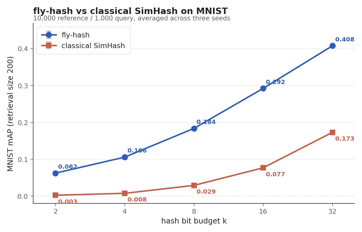
fly-hash beats classical SimHash at every hash-bit budget. The gap is largest when you have only a few bits to spend. Averaged over three random seeds.
| hash bits | fly-hash | classical SimHash | fly beats by |
|---|---|---|---|
| 2 | 0.062 | 0.003 | 26x |
| 4 | 0.106 | 0.008 | 14x |
| 8 | 0.184 | 0.029 | 6.5x |
| 16 | 0.292 | 0.077 | 3.9x |
| 32 | 0.408 | 0.173 | 2.4x |
fly-hash wins at every bit budget (higher is better). The biggest margin is at the smallest budgets, where you have to squeeze a handwritten digit into just two or four bits of identity. At 32 bits, classical SimHash finally starts to tell 200 MNIST digits apart with some skill. Fly-hash is still more than twice as good.
My graphed numbers are slightly steeper than the paper’s, but the shape of the curve and the conclusion are the same. The gap comes from small choices the paper does not specify exactly (retrieval size, tie-breaking, preprocessing), and I checked that twiddling those does not change which hash wins.
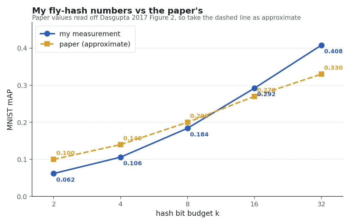
My measured fly-hash mAP against the paper’s reported numbers on MNIST. The paper’s values are eyeballed from its Figure 2 and should be treated as approximate. My curve is a little steeper at the low-bit end and a little higher at the high-bit end, but the rank order, the direction, and the fly-beats-classical story are the same.
That is what I wanted to see. Not a cycle-accurate replication, but proof that the algorithm actually does what the paper claims on a real dataset I made up, against a real baseline. Expansion plus winner-take-all is a genuinely better way to do nearest-neighbor hashing when you have very few bits to spend. That fact survives reproduction. Good.
Now Put It on a Commodore 64
You knew this was coming, right?
Vogelstein’s 2025 paper uses a 3,000-neuron connectome and trains input and output layers with PyTorch on a modern GPU. None of that fits on a Commodore 64. But the 2017 fly-hash, shrunk down to 500 Kenyon cells and 20 reference patterns, absolutely does. (A “reference pattern” here is one of the twenty toy bitmaps shown earlier in the article — think of them as the tiny library of known smells the C64 will compare new inputs against.)
This is not a gimmick, and it is not a sidenote. Running an algorithm on a computer that is a million times slower than your laptop forces you to understand it completely. You cannot hide behind import numpy or torch.nn.Linear or the Metal GPU in my Macs that run 4.26 TFLOPS (trillion floating-point operations per second).
The Commodore 64’s 6510 CPU at ~1 MHz can, at best, perform about 300,000 operations per second, and we only have 64k of RAM. Every byte of RAM has a reason. Every inner-loop instruction gets counted. By the time the thing runs on a 1 MHz 6510, you know exactly what the Mac GPU was doing for you for free, which is most of the algorithm.
There is a second reason, which I will come back to at the end. The memory and compute footprint that the C64 forces on you is similar to that of the 50-cent embedded microcontrollers made in the last fifteen years. If the fly-brain algorithm works at C64 scale, it works on a two-dollar chip you can solder to a breadboard and run off a battery for a month. That is the difference between an interesting paper and a deployable product.
So. A 1982 home computer running an algorithm from a 2017 Science paper, in the same research tradition as a 2025 Johns Hopkins paper trying to build artificial intelligence on a fruit fly’s brain. The article will exist either way. I want it to actually do the thing, not just talk about it.
Are YOU keeping up with the Commodore?
Here is the memory budget at the scale I picked:
| thing | bytes |
|---|---|
| projection (500 cells × 6 indices) | 3,000 |
| 20 reference patterns (50 bits each) | 1,000 |
| 20 reference hashes (25 active each) | 500 |
| working arrays | ~2,000 |
| program code | ~1,000 |
Under 8 KB of core data in a machine with 38,911 bytes free after BASIC loads. Pretty comfortable.
The projection and reference hashes get generated on my desktop once and exported as BASIC DATA statements. The Python side writes files like:
REM FLY-HASH PROJECTION: 500 KENYON CELLS X 6 INPUTS EACH
REM 3000 BYTES TOTAL, INDICES 0..49
10000 DATA 1,7,14,15,17,40,5,6,8,34,43,47,1,2,5,13
10010 DATA 41,49,23,24,30,46,7,15,18,26,32,42,...
The C64 reads that with READ into an integer array and off we go.
The hash loop in Commodore BASIC V2 is a direct translation of the Python:
1000 REM HASH PATTERN P INTO QT
1010 FOR K=0 TO NK-1
1020 AC%(K)=PAT%(P,PR%(K,0))+PAT%(P,PR%(K,1))+PAT%(P,PR%(K,2))
1030 AC%(K)=AC%(K)+PAT%(P,PR%(K,3))+PAT%(P,PR%(K,4))+PAT%(P,PR%(K,5))
1040 NEXT K
1050 REM WINNER-TAKE-ALL
1060 FOR W=0 TO NW-1
1070 MX=-1:KX=-1
1080 FOR K=0 TO NK-1
1090 IF AC%(K)>MX THEN MX=AC%(K):KX=K
1100 NEXT K
1110 QT%(W)=KX
1120 AC%(KX)=-1
1130 NEXT W
1140 RETURN
PR%(K,S) is the input dimension that the S-th sample of Kenyon cell K looks at. PAT%(P,D) is bit D of pattern P. AC%(K) is the sum for Kenyon cell K. The winner-take-all loop finds the maximum, writes it to the output tag, blanks it out with -1, and repeats 25 times.
For you Commodore nerds now yelling at me: Integer variables with % are actually slower than floats in BASIC V2, because the interpreter converts them back to floats for every arithmetic operation. I used them anyway because they halve the array memory, which matters more than speed here.
Running It
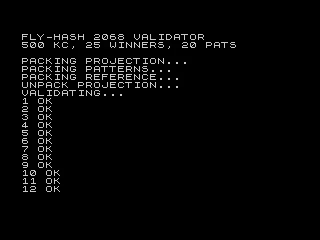
Time to run the thing. Let’s get the BASIC program into the C64 and let it start crunching.
The OK after each pattern number is doing real work. The Python reference generator pre-computes what the 25 winner indices should be for each of the 20 patterns, writes them into BASIC DATA statements, and the C64 compares its own hash against those reference indices pattern by pattern. OK means every single winner index matched the Python reference. 20 OKs means the 6510 and my laptop agree on all 500 winner-cell decisions.
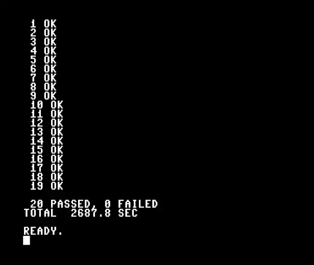
Stock C64 running the fly-hash on all 20 reference patterns. 20 passed, 0 failed. About 45 minutes from RUN to READY on a 1 MHz 6510.
Forty-five minutes on a real 1 MHz 6510 is a long time to watch a demo. Load the program, type RUN, go make coffee, come back, and the last pattern is just being checked. That is why the next version of this code is written in 6502/10 assembly. The projection loop and the winner-take-all loop together account for almost all of those 45 minutes, and both translate cleanly to native 6502.
Making It Fast
BASIC V2 is slow. Every single line of BASIC, every loop iteration, every array access, gets interpreted from a tokenized program representation, routed through a pile of generic code paths, and translated through the floating-point unit even when it doesn’t need to be. The hash’s inner loop does roughly three thousand pattern-byte lookups plus three thousand additions per pattern, and the winner-take-all does twelve thousand comparisons. Multiply by the interpretation overhead and you get 45 minutes.
The fix is to do the hot loops in native 6502 assembly and leave BASIC in charge of everything else. BASIC still loads the projection, references, and patterns from DATA into fixed memory addresses. BASIC still drives the outer loop and prints results. But the inner work happens in about 460 bytes of hand-written machine code at $C000, called from BASIC with SYS 49152 once per pattern.
Here is the projection kernel in 6502, which replaces BASIC lines 1020-1030. The two additional lines in BASIC sum six pattern bytes through a layer of array-index arithmetic; the assembly dereferences two pointers directly and skips the floating-point unit entirely:
project_loop:
    ldy #0
    lda (proj_ptr),y     ; read the 0th input index for this Kenyon cell
    tay                  ; y = that index (0..49)
    lda (pat_ptr),y      ; a = pattern[index] (0 or 1)
    sta temp_sum
    ldy #1
    lda (proj_ptr),y
    tay
    lda (pat_ptr),y
    clc
    adc temp_sum
    sta temp_sum
    ; ... four more unrolled iterations for samples 2..5 ...
    clc
    adc #1               ; +1 so 0 can be the "already picked" sentinel
    ldy #0
    sta (act_ptr),y      ; activations[cell] = sum + 1
    ; advance proj_ptr by 6, act_ptr by 1, decrement cell_count, branch
Zero floats. Zero BASIC interpretation. Every instruction is a single or double-byte opcode, executed in 2 to 5 clock cycles on the 6510.
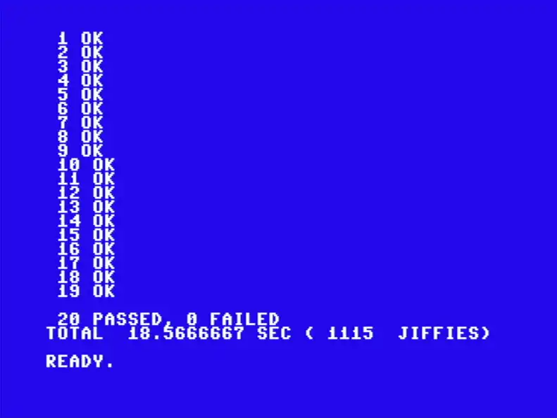
Same 20 patterns, same reference hashes, same algorithm. 18.57 seconds instead of 45 minutes. The 6502 inner loop fits in 465 bytes.
Twenty passed, zero failed, 18.57 seconds. A hundred and forty-five times faster than BASIC, and the assembly is not even tuned. The winner-take-all is still a naive O(n) scan done twenty-five times, and the projection still uses 16-bit address arithmetic everywhere.
The algorithm from a 2017 science paper is now a demo you can *use on a forty-three-year-old computer powered by a processor less powerful than your Apple Watch by a huge margin.
Pushing to MNIST Scale with an REU
The 20-pattern demo is a proof that the algorithm works. It is not proof that the algorithm is useful. For that I want real data: thousands of handwritten digits from MNIST, indexed by fly-hash, retrieved by the C64 itself. But the arithmetic for that is cruel. Ten thousand MNIST references, each hashed to 25 winner cell indices stored as 16-bit integers, is half a megabyte of reference tags alone. A stock Commodore 64 has 64 KB of RAM total, most of it unavailable once BASIC loads.
Commodore shipped a solution in 1985: the RAM Expansion Unit, or REU. It is a cartridge stuffed with extra RAM chips plus a built-in copier called a DMA controller. DMA stands for “direct memory access,” and the idea is that the cartridge can move a chunk of its own memory into the Commodore 64’s main memory in one request, without the main CPU having to ferry each byte by hand. That is the only way the arithmetic works on a 1 MHz chip. The original REU held at most 512 KB, but modern drop-in replacements, such as the Ultimate 1541-II+, have an REU that emulates original Commodore hardware from the C64’s perspective.
I can hear the purists screaming, but just hang with me here. I want to demonstrate that a simple computer can do this work without getting caught up in religious wars.
So my REU sizes up to 16 MB, and I can preload content from an SD card at boot. For our purposes, 16 MB is plenty to hold:
- the 500-Kenyon-cell projection matrix (6 KB)
- ten MNIST test digits (8 KB)
- ten thousand reference digit hashes (500 KB)
- ten thousand ground-truth labels (10 KB)
All generated on the Mac, serialized into a 16 MB binary blob, and copied to an SD card, the Ultimate II+ reads on boot.
The C64 side is a new BASIC driver that calls a new 881-byte 6502 routine at $C000. For each of the ten pre-loaded test digits, the assembly:
- DMAs the query image from REU into C64 RAM, binarizes the pixels
- Hashes it with the same 500-cell, 25-winner fly-hash
- Builds a 63-byte bitmap of the query’s winner cells
- DMAs each of the 10,000 reference hashes one at a time, counts bitmap overlaps, and maintains a top-5 leaderboard
- DMAs the five winning labels from the REU’s labels region
- Returns to BASIC, which prints one row of the results table
Total per query: 28 seconds on a real 1 MHz 6510, dominated by the 10,000 REU-to-C64 reads of 50 bytes each. The full ten-query run is under five minutes.
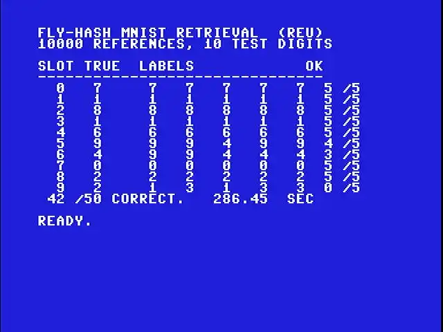
Real MNIST retrieval on a real Commodore 64 with a 16 MB REU. For each of ten pre-loaded test digits, the C64 hashes the digit and returns the five most-similar references out of ten thousand. 42 of 50 top-5 predictions match the query’s true label.
Slot 0 is a handwritten “7”. The C64 hashes it, walks all 10,000 references in the REU, and returns five references the fly-hash says are most similar. All five are labeled “7”. Same clean 5-for-5 on slots 1 through 4. Slot 5 retrieves four 9s and one 4 for a “9” query — close. Slot 6 is harder (the “4” retrieves as 4, 4, 4, 9, 9 — three right). Slot 9 is the genuinely hard one. It’s a weird-looking “2” that gets pulled back as 1, 3, 1, 3, 3. Zero out of five.
84% top-5 accuracy on real MNIST, from a forty-three-year-old computer and an expansion cartridge designed when the paper this implements would not exist for another three decades.
Neat-O.
What the C64 Actually Proved
Step back from the 1982 aesthetic for a second (or don’t, I’ve not stopped loving it). The whole classifier, twenty reference patterns plus a 500-Kenyon-cell projection, fits in about 8 KB of data and another 2 KB of code. That footprint comfortably fits in an ATmega328, which is the chip inside an Arduino Uno. It fits in an ESP32, which is a dollar-and-a-half Wi-Fi-capable microcontroller. It fits in any of two dozen microcontroller families that run at around 160 MHz and draw tenths of a watt.
160 MHz is roughly 160 times faster than the C64. And add that a modern 32-bit core does about 6 times as much work per clock as a 6510, and it’s about 1000x faster. The same algorithm, at the same scale we just proved correct, would run in a few seconds on a thing you can put on a breadboard and power with a battery for a month.
The Commodore 64 is the showpiece. The microcontroller running the same algorithm is a real chip you can buy today, and cheap.
So, what would you actually do with that chip?
Where a BPU Earns Its Keep
Nobody is going to use a BPU to write code or summarize PDFs. The useful question is where the LLM architecture cannot go, and what a fly-brain-sized network might do once it arrives there.
Here are three examples:
On-orbit image triage. A cubesat (a small standardized satellite, each unit a 10-cm cube, often no bigger than a shoebox) in low orbit, with a power budget for Earth orbit, has a camera at single-digit watts. Downlink bandwidth is scarce and expensive. You don’t want to downlink every frame. You want the spacecraft to classify on board: ship or no ship, smoke plume or shadow, new road since last pass or not. An LLM does not fit in the spacecraft’s RAM, let alone run on the power a small coin cell would laugh at. A BPU is the right size for this job by two orders of magnitude. This is the reason DARPA started O-CIRCUIT in the first place.
Wearable health. A smart ring or watch that continuously classifies what you’re doing (walking, running, sitting, falling down, sleeping badly, having a heart event) needs to run for a week on a battery and cannot depend on your phone having a signal. The classifier has to be tiny, fast, and rugged. Most of the modern wearable ecosystem cheats by offloading inference to a phone or the cloud. A BPU-sized classifier doesn’t need to cheat.
Smell. The fly’s circuit we just spent an article replicating is literally a smell classifier. It is good at nearest-neighbor-style “is this like any of these reference things” problems because that is the problem it evolved to solve. Point a small electronic nose at an industrial pipeline and have it continuously sniff for the 200 volatile organic compounds that mean “leak.” Point it at a cargo container and have it notice cocaine or fentanyl. Point it at a loaf of bread in a grocery supply chain and have it call out the beginnings of mold. This is a market with real dollars behind it that current AI has not broken in to, partly because LLMs are the wrong shape for it. The algorithm we ran on the Commodore 64 is closer to the right shape than any of the frontier models.
None of those places can host a frontier LLM. None of them has any business uplinking every detection to the cloud. A fly-hash of this size fits, runs, and gives you a useful classification.
I’m sure if we sit here for 20 minutes we could come up with hundreds of ideas where this would be useful together.
I triple dog dare you.
Just for Fun: The Same Algorithm on a Timex 2068
A friend of mine had a Timex Sinclair 2068 as a kid and cut his first programming teeth on it. He brought that up last week, and the idea of putting the fly-hash on a 2068 stuck. After a couple of days hanging out with him, I traded a spare TI-99/4A to get my hands on a real 2068 of my own. Same scope as the C64 demo, same reference data, same 500 Kenyon cells, same 20 patterns. Different processor (Z80 instead of 6510) and a different BASIC dialect.
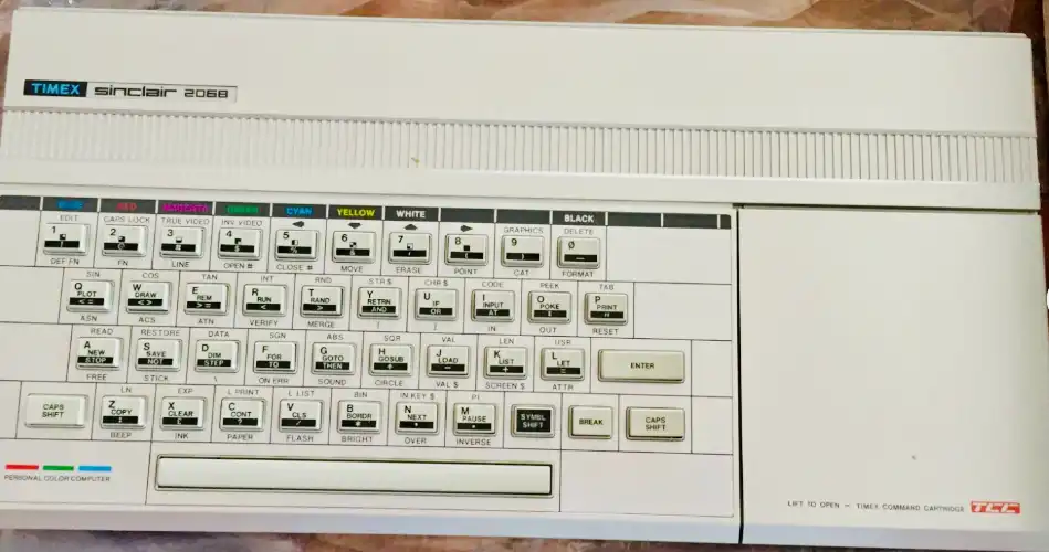
My Timex Sinclair 2068. Look at the keys. Every one of them has three or four legends printed on it for the different shift modes. PRINT lives on the P key, OR lives on the U key, GO TO is on G, and so on. That is what BASIC entry looks like on this machine.
I should say up front that I find the Sinclair-style keyboard input model nearly impossible to use. On a real 2068 (and the Spectrum it descends from), you do not type BASIC keywords letter by letter. Each key is overloaded with a whole keyword that gets entered as a single token, and which keyword you get depends on which of several shift modes the editor is in. Pressing P in the right mode gives you PRINT. Pressing it in a different mode gives you the letter P. Coming from a Commodore keyboard, where every keystroke is just the character on the cap, it feels like trying to type with mittens on.
The trouble started with memory. Sinclair BASIC stores every numeric value in a DATA statement as ASCII text and a hidden 5-byte float. A 500-by-6 numeric array eats 15 KB on its own. The full set of weights, as DATA statements, comes to about 63 KB. The 2068 has roughly 41 KB free for BASIC. It does not fit.
So the data goes into strings instead, packed as CHR$ codes:
- The 3,000 projection indices become 3,000 single characters in
A$. Each character isCHR$(35 + value), which keeps every byte within printable ASCII and avoids the double quote. - The 1,000 pattern bits are literally
'0'and'1'inB$. - The 500 reference indices need two characters each (since they go up to 499) and live in
C$as base-90 pairs.
That gets the data down from about 35 KB unpacked to 5 KB packed. The whole thing fits, with about 13 KB to spare for working arrays.
Sinclair BASIC has its own quirks. Arrays are 1-indexed instead of 0-indexed. LET is mandatory on every assignment. The screen pauses with a scroll? prompt every 22 lines unless you POKE 23692,255 to keep the counter cranked up. None of these are hard; they just have to be reckoned with.
The result: 20 out of 20 patterns match the reference hashes. Same answer the C64 produced, on a different chip family, in a different BASIC dialect.
Timex 2068 chewing through the 20 patterns. Twelve in, eight to go. No scroll prompt thanks to POKE 23692,255.
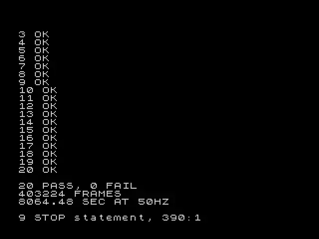
20 PASS, 0 FAIL. 403,224 frames at 50 Hz is 8,064 seconds, which works out to a little over two and a quarter hours.
The Timex BASIC is not faster than the Commodore BASIC. In fact, it’s slower by a good margin. At least my implementation is. I’m sure there are Spectrum people screaming at me right now. Calm down. The same algorithm at the same scale took 45 minutes in Commodore BASIC on a 1 MHz 6510, and a little over 2 hours in Sinclair BASIC on a 3.5 MHz Z80. Interpreted BASIC is so heavy that the extra clock speed disappears into floating-point arithmetic and 2D array indexing overhead. A Z80 assembly version would be the natural sequel, in keeping with the symmetry of the 6502 port. That is a job for another weekend if I can stomach this keyboard for one more minute.
What This Is Warming Up For
This article is Phase 0 of a bigger project. My next quest is the actual Vogelstein 2025 paper: 3,016 larva neurons, MNIST digit recognition, plus CIFAR (basically MNIST-but-harder: small color photos of ten object categories like airplane, cat, and truck). Running on my Mac mini’s built-in GPU, which is fast enough to train the whole thing at home in a few hours. That is where biology-as-substrate begins to do real classification work on real datasets.
After that, the open question is whether more biology buys more performance. The adult fruit fly’s full wiring diagram was recently mapped by the FlyWire project — 139,000 neurons, roughly fifty times the size of the larva’s. Does the bigger substrate pick up harder tasks? Does it help at all? Someone has to check.
Dasgupta, Stevens, and Navlakha did the hard part in 2017. I just translated their algorithm to two 1980s chips and confirmed the answer still comes out right.
The Commodore 64 and Timex 2068 do not solve any of those open problems. What they do is prove I can hold the algorithm in my hand and see it move, on the slowest substrates I care about. The 1982 machines teach me what the 2025 paper is actually doing in a way that reading a PDF never will. When you make an algorithm run on a computer that does one thing per microsecond, you understand it in a way a GPU never lets you.
That is the whole point of retro computing, at least for me. It is also why I am willing to spend weekends on this kind of thing. LLMs won the last decade on the bet that scale plus data can substitute for structure. BPUs are a bet that for the problems a data center cannot reach, six hundred million years of evolution still beats last year’s GPU allocation. Both bets can be right at the same time. The second one is the one I want to live in for a while.
So I loaded the demo on a real C64, typed RUN, and watched a 1982 computer do what a fruit fly does. Then I did it again on a Timex. Pretty neat for a weekend project.
Glossary
Terms that show up in this piece without a full definition, for anyone (me included) using this as a study guide. The five most essential terms (parameter, gradient descent, vector/dimension, inhibitory neuron, MNIST) are glossed inline where they first appear. Everything below is the supplement.
Sparse random projection. The first step of the fly-hash. Each output cell (“Kenyon cell”) only looks at a small random handful of the inputs, not all of them. “Random” because which inputs get looked at is chosen once with a random number generator and frozen forever. “Sparse” because the handful is small: about 10% of the inputs in the paper, fewer in smaller versions.
Winner-take-all. A general neural-circuit pattern where a group of competing cells silences all but the strongest few. In the fly’s mushroom body, the APL neuron implements an approximate winner-take-all across the ~2,000 Kenyon cells, leaving about 5% active. In machine learning, the same pattern shows up under names like “top-k,” “k-sparse coding,” and “lateral inhibition.”
Kenyon cells/mushroom body. The mushroom body is a paired structure near the top of the fly’s brain, named after its shape. Its principal neurons are the Kenyon cells, named after Frederick Kenyon, who identified them in 1896. They are where the fly stores odor memories, and where the 2017 paper’s entire argument lives.
Substrate. The physical or structural thing actually doing the computing. Silicon is the substrate of a CPU. Transformer weights are the substrate of an LLM. The fly connectome is the substrate of a BPU. The distinction matters because the same algorithm can run on different substrates (with very different power and size costs), and a different algorithm on the same substrate can make a completely different machine.
Transformer. The neural-network architecture behind every LLM you know. Its one distinctive move is “attention”: each token in the input (word, pixel, whatever) gets to look at every other token and decide how much it cares about each. The results are combined, passed through a few standard layers, and handed to the next attention block. Repeat dozens of times, and that is GPT. Introduced in a 2017 Google paper called Attention Is All You Need.
Large language model (LLM). A transformer trained on enormous amounts of text (books, web pages, code) to predict the next word given the preceding words. That one objective, at sufficient scale, produces systems that can summarize, translate, write code, and chat. ChatGPT, Claude, Gemini, Llama all belong to this category.
Connectome. A complete wiring diagram of a nervous system: every neuron, every synapse, every direction of every connection, mapped out from electron microscopy reconstructions. The fruit fly larva was the first whole-animal brain connectome, published by Winding et al. in 2023. The adult fly followed via the FlyWire project.
Nearest-neighbor retrieval. Given a query item and a database of reference items, return the references most similar to the query. “Similar” could mean lowest Euclidean distance, highest cosine similarity, fewest differing bits, whatever the problem needs. The engine behind image search, song identification, recommendation systems, and plagiarism detection.
Edge compute. Any computation that happens close to where the data is generated, without shipping it off to a cloud data center. A smart thermostat inferring “you are home” from a motion sensor is edge compute. A satellite classifying images on-orbit is edge compute. Anything that cannot rely on network connectivity counts, and anything that has to run on a battery mostly has to run this way.
Spectral radius. The largest magnitude among the eigenvalues of a matrix. Not in this article, but it will come up in the next one: reservoirs need their recurrent weight matrix to have a spectral radius below 1 to avoid “exploding dynamics” where the signal grows without bound when the network is iterated.
Reservoir / reservoir computing. Also not in this article. A neural-network architecture where a large recurrent middle layer is fixed at initialization and only the input and output projections are trained. The BPU is a reservoir whose middle happens to be a real fruit fly brain instead of a random matrix.