Sorting Algorithms Visualized on the Commodore 64
One of the best ways to understand how sorting algorithms work is to watch them run. Modern computers are too fast—everything happens in a blink. But on an 8-bit machine running BASIC? You can watch every comparison, every swap, every decision the algorithm makes.
We’ll implement three classic sorting algorithms on the Commodore 64, visualizing each as an animated bar chart using PETSCII characters.
The Setup: PETSCII Bar Charts
All three programs share the same visualization approach: an array of random values displayed as vertical bars on screen. As the algorithm sorts, you can watch the bars rearrange themselves in real-time.
Each program includes two subroutines starting at line 500:
- Lines 500-595: Draw all bars (used for initial display)
- Lines 600-680: Redraw a single bar at position X1 (used during sorting)
Bars are drawn from the bottom of the screen upward using POKE to screen memory (1024) and color memory (55296). The height of each bar corresponds to its value, and colors indicate the algorithm’s current state—yellow for comparing, red for swapping, green for sorted.
Bubble Sort: The Friendly Neighbor
Bubble sort is the simplest sorting algorithm. It repeatedly steps through the list, compares adjacent elements, and swaps them if they’re in the wrong order. Larger values “bubble up” to the end of the list.
10 REM BUBBLE SORT VISUALIZER FOR C64
15 REM MICHAEL DOORNBOS 2025
20 PRINT CHR$(147):REM CLEAR SCREEN
30 POKE 53280,0:POKE 53281,0:REM BLACK BORDER/BACKGROUND
40 N=18:DIM A(N):REM 18 ELEMENTS
50 REM INITIALIZE WITH RANDOM VALUES
60 FOR I=0 TO N-1
70 A(I)=INT(RND(1)*20)+1
80 NEXT I
90 CL=14:GOSUB 500:REM DRAW INITIAL BARS IN LIGHT BLUE
95 PRINT CHR$(19);"BUBBLE SORT - PRESS ANY KEY"
96 GET K$:IF K$="" THEN 96
98 TI$="000000"
100 REM BUBBLE SORT
110 FOR I=N-1 TO 1 STEP -1
120 SW=0:REM SWAP FLAG
130 FOR J=0 TO I-1
140 REM HIGHLIGHT COMPARING ELEMENTS
150 CL=7:X1=J:GOSUB 600:REM YELLOW
160 CL=7:X1=J+1:GOSUB 600
170 FOR D=1 TO 50:NEXT:REM DELAY
180 IF A(J)<=A(J+1) THEN 240
190 REM SWAP
200 T=A(J):A(J)=A(J+1):A(J+1)=T
210 SW=1
220 CL=2:X1=J:GOSUB 600:REM RED FLASH FOR SWAP
230 CL=2:X1=J+1:GOSUB 600
235 FOR D=1 TO 30:NEXT
240 REM RESTORE COLOR
250 CL=14:X1=J:GOSUB 600
260 CL=14:X1=J+1:GOSUB 600
270 NEXT J
280 REM MARK SORTED ELEMENT GREEN
290 CL=5:X1=I:GOSUB 600
300 IF SW=0 THEN 330:REM EARLY EXIT IF NO SWAPS
310 NEXT I
320 CL=5:X1=0:GOSUB 600:REM FIRST ELEMENT
330 PRINT CHR$(19);"BUBBLE SORT - DONE IN"TI/60"SECONDS"
340 GET K$:IF K$="" THEN 340
350 END
500 REM DRAW ALL BARS
510 FOR I=0 TO N-1
520 X=I*2+2
530 FOR Y=24 TO 24-A(I)+1 STEP -1
540 POKE 1024+Y*40+X,160:POKE 55296+Y*40+X,CL
550 NEXT Y
560 FOR Y=24-A(I) TO 1 STEP -1
570 POKE 1024+Y*40+X,32
580 NEXT Y
590 NEXT I
595 RETURN
600 REM DRAW SINGLE BAR AT X1
610 X=X1*2+2
620 FOR Y=24 TO 24-A(X1)+1 STEP -1
630 POKE 1024+Y*40+X,160:POKE 55296+Y*40+X,CL
640 NEXT Y
650 FOR Y=24-A(X1) TO 1 STEP -1
660 POKE 1024+Y*40+X,32
670 NEXT Y
680 RETURN
The Commodore screen grabs are all running at 20x speed…
How Bubble Sort Works:
- Compare adjacent elements from left to right
- Swap if the left element is larger than the right
- Repeat passes until no swaps are needed
- After each pass, the largest unsorted element “bubbles” to its final position
What You’ll See:
- Yellow highlights show the two elements being compared
- Red flashes indicate a swap
- Green marks elements in their final sorted position
- The algorithm naturally slows down as it finishes (fewer swaps needed)
Time Complexity: O(n²) average and worst case, but O(n) best case if already sorted (thanks to the early exit optimization).
Without Visualization
Strip away the graphics and you get the pure algorithm. This version sorts 100 elements so you can measure actual sort time:
10 REM BUBBLE SORT - NO VISUALIZATION
15 REM MICHAEL DOORNBOS 2025
20 PRINT CHR$(5):PRINT CHR$(147);"BUBBLE SORT BENCHMARK"
30 N=100:DIM A(N)
40 FOR I=0 TO N-1:A(I)=INT(RND(1)*1000):NEXT
50 PRINT "SORTING";N;"ELEMENTS..."
60 TI$="000000"
70 FOR I=N-1 TO 1 STEP -1
80 SW=0
90 FOR J=0 TO I-1
100 IF A(J)<=A(J+1) THEN 130
110 T=A(J):A(J)=A(J+1):A(J+1)=T:SW=1
130 NEXT J
140 IF SW=0 THEN 160
150 NEXT I
160 PRINT "DONE IN";TI/60;"SECONDS"
Result: 100.72 seconds on a real C64.
Selection Sort: The Methodical Picker
Selection sort divides the array into sorted and unsorted regions. It repeatedly finds the minimum element from the unsorted region and moves it to the end of the sorted region.
10 REM SELECTION SORT VISUALIZER FOR C64
15 REM MICHAEL DOORNBOS 2025
20 PRINT CHR$(147):REM CLEAR SCREEN
30 POKE 53280,0:POKE 53281,0
40 N=18:DIM A(N)
50 REM INITIALIZE WITH RANDOM VALUES
60 FOR I=0 TO N-1
70 A(I)=INT(RND(1)*20)+1
80 NEXT I
90 CL=14:GOSUB 500:REM DRAW INITIAL BARS
95 PRINT CHR$(19);"SELECTION SORT - PRESS ANY KEY"
96 GET K$:IF K$="" THEN 96
98 TI$="000000"
100 REM SELECTION SORT
110 FOR I=0 TO N-2
120 MN=I:REM ASSUME FIRST IS MINIMUM
130 CL=3:X1=I:GOSUB 600:REM CYAN FOR CURRENT POSITION
140 FOR J=I+1 TO N-1
150 REM HIGHLIGHT ELEMENT BEING CHECKED
160 CL=7:X1=J:GOSUB 600:REM YELLOW
170 FOR D=1 TO 30:NEXT
180 IF A(J)>=A(MN) THEN 210
190 REM NEW MINIMUM FOUND
200 IF MN<>I THEN CL=14:X1=MN:GOSUB 600:REM RESTORE OLD MIN
205 MN=J:CL=2:X1=MN:GOSUB 600:REM RED FOR NEW MIN
206 GOTO 220
210 CL=14:X1=J:GOSUB 600:REM RESTORE TO BLUE
220 NEXT J
230 REM SWAP MINIMUM WITH POSITION I
240 IF MN<>I THEN T=A(I):A(I)=A(MN):A(MN)=T
250 REM REDRAW SWAPPED ELEMENTS
260 CL=14:X1=MN:GOSUB 600
270 CL=5:X1=I:GOSUB 600:REM GREEN FOR SORTED
280 NEXT I
290 CL=5:X1=N-1:GOSUB 600:REM LAST ELEMENT
300 PRINT CHR$(19);"SELECTION SORT - DONE IN"TI/60"SECONDS"
310 GET K$:IF K$="" THEN 310
320 END
500 REM DRAW ALL BARS
510 FOR I=0 TO N-1
520 X=I*2+2
530 FOR Y=24 TO 24-A(I)+1 STEP -1
540 POKE 1024+Y*40+X,160:POKE 55296+Y*40+X,CL
550 NEXT Y
560 FOR Y=24-A(I) TO 1 STEP -1
570 POKE 1024+Y*40+X,32
580 NEXT Y
590 NEXT I
595 RETURN
600 REM DRAW SINGLE BAR AT X1
610 X=X1*2+2
620 FOR Y=24 TO 24-A(X1)+1 STEP -1
630 POKE 1024+Y*40+X,160:POKE 55296+Y*40+X,CL
640 NEXT Y
650 FOR Y=24-A(X1) TO 1 STEP -1
660 POKE 1024+Y*40+X,32
670 NEXT Y
680 RETURN
How Selection Sort Works:
- Find the minimum element in the unsorted region
- Swap it with the first unsorted element
- Expand the sorted region by one
- Repeat until the entire array is sorted
What You’ll See:
- Cyan marks the position we’re filling
- Yellow scans through unsorted elements
- Red marks the current minimum found
- Green shows the growing sorted region on the left
Time Complexity: Always O(n²)—it always scans the full unsorted region, even if already sorted. However, it minimizes swaps (at most n-1).
Without Visualization
10 REM SELECTION SORT - NO VISUALIZATION
15 REM MICHAEL DOORNBOS 2025
20 PRINT CHR$(5):PRINT CHR$(147);"SELECTION SORT BENCHMARK"
30 N=100:DIM A(N)
40 FOR I=0 TO N-1:A(I)=INT(RND(1)*1000):NEXT
50 PRINT "SORTING";N;"ELEMENTS..."
60 TI$="000000"
70 FOR I=0 TO N-2
80 MN=I
90 FOR J=I+1 TO N-1
100 IF A(J)>=A(MN) THEN 120
110 MN=J
120 NEXT J
130 IF MN=I THEN 150
140 T=A(I):A(I)=A(MN):A(MN)=T
150 NEXT I
160 PRINT "DONE IN";TI/60;"SECONDS"
Result: 47.25 seconds on a real C64.
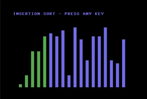
Insertion Sort: The Card Player
Insertion sort works like sorting a hand of cards. You pick up cards one at a time and insert each into its proper position among the cards you’ve already sorted.
10 REM INSERTION SORT VISUALIZER FOR C64
15 REM MICHAEL DOORNBOS 2025
20 PRINT CHR$(147):REM CLEAR SCREEN
30 POKE 53280,0:POKE 53281,0
40 N=18:DIM A(N)
50 REM INITIALIZE WITH RANDOM VALUES
60 FOR I=0 TO N-1
70 A(I)=INT(RND(1)*20)+1
80 NEXT I
90 CL=14:GOSUB 500:REM DRAW INITIAL BARS
95 PRINT CHR$(19);"INSERTION SORT - PRESS ANY KEY"
96 GET K$:IF K$="" THEN 96
98 TI$="000000"
110 FOR I=1 TO N-1
120 KY=A(I):REM KEY TO INSERT
130 CL=7:X1=I:GOSUB 600:REM HIGHLIGHT KEY IN YELLOW
140 FOR D=1 TO 50:NEXT
150 J=I-1
160 REM SHIFT ELEMENTS RIGHT
170 IF J<0 THEN 250
180 IF A(J)<=KY THEN 250
190 REM SHIFT ELEMENT RIGHT
200 CL=2:X1=J:GOSUB 600:REM RED FOR SHIFTING
210 FOR D=1 TO 30:NEXT
220 A(J+1)=A(J)
230 CL=14:X1=J+1:GOSUB 600:REM REDRAW SHIFTED
240 J=J-1:GOTO 170
250 REM INSERT KEY
260 A(J+1)=KY
270 CL=5:X1=J+1:GOSUB 600:REM GREEN FOR INSERTED
280 FOR D=1 TO 30:NEXT
285 REM SHOW SORTED PORTION
286 FOR K=0 TO I:CL=5:X1=K:GOSUB 600:NEXT
290 NEXT I
300 PRINT CHR$(19);"INSERTION SORT - DONE IN"TI/60"SECONDS"
310 GET K$:IF K$="" THEN 310
320 END
500 REM DRAW ALL BARS
510 FOR I=0 TO N-1
520 X=I*2+2
530 FOR Y=24 TO 24-A(I)+1 STEP -1
540 POKE 1024+Y*40+X,160:POKE 55296+Y*40+X,CL
550 NEXT Y
560 FOR Y=24-A(I) TO 1 STEP -1
570 POKE 1024+Y*40+X,32
580 NEXT Y
590 NEXT I
595 RETURN
600 REM DRAW SINGLE BAR AT X1
610 X=X1*2+2
620 FOR Y=24 TO 24-A(X1)+1 STEP -1
630 POKE 1024+Y*40+X,160:POKE 55296+Y*40+X,CL
640 NEXT Y
650 FOR Y=24-A(X1) TO 1 STEP -1
660 POKE 1024+Y*40+X,32
670 NEXT Y
680 RETURN
How Insertion Sort Works:
- Take the next unsorted element (the “key”)
- Compare it with sorted elements from right to left
- Shift larger elements one position right
- Insert the key in its correct position
- Repeat until all elements are processed
What You’ll See:
- Yellow highlights the element being inserted
- Red shows elements shifting right to make room
- Green grows from left as the sorted region expands
Time Complexity: O(n²) worst case, but O(n) best case for nearly-sorted data. This makes it excellent for data that’s “almost sorted.”
Without Visualization
10 REM INSERTION SORT - NO VISUALIZATION
15 REM MICHAEL DOORNBOS 2025
20 PRINT CHR$(5):PRINT CHR$(147);"INSERTION SORT BENCHMARK"
30 N=100:DIM A(N)
40 FOR I=0 TO N-1:A(I)=INT(RND(1)*1000):NEXT
50 PRINT "SORTING";N;"ELEMENTS..."
60 TI$="000000"
70 FOR I=1 TO N-1
80 KY=A(I):J=I-1
90 IF J<0 THEN 120
100 IF A(J)<=KY THEN 120
110 A(J+1)=A(J):J=J-1:GOTO 90
120 A(J+1)=KY
130 NEXT I
140 PRINT "DONE IN";TI/60;"SECONDS"
Result: 47.33 seconds on a real C64.
Comparing the Three
Each algorithm has a distinct visual personality:
| Algorithm | Visual Pattern | Best For |
|---|---|---|
| Bubble Sort | Ripples from left to right, large values float up | Educational purposes, small datasets |
| Selection Sort | Scans right, builds sorted region left | When swaps are expensive |
| Insertion Sort | Shifts and inserts, sorted region grows left | Nearly-sorted data, online sorting |
Real C64 Benchmark Results
Running the non-visualized versions on actual hardware (100 elements):
| Algorithm | Time (seconds) |
|---|---|
| Bubble Sort | 100.72 |
| Selection Sort | 47.25 |
| Insertion Sort | 47.33 |
Bubble sort takes more than twice as long as the others. Even though all three are O(n²), bubble sort’s constant factor is higher—it does more swaps, moving elements one position at a time instead of finding the right spot first.
What to Watch For
Bubble Sort creates a mesmerizing ripple effect. Watch how larger values seem to float toward the right side with each pass. The green “done” region grows from the right.
Selection Sort is methodical and predictable. Each pass does exactly one swap (at most). The green region grows steadily from the left, one element at a time.
Insertion Sort has the most dynamic movement. Elements shift like cards in a hand, making room for each new insertion. Nearly-sorted arrays finish quickly because fewer shifts are needed.
Understanding Time Complexity
When we talk about algorithm efficiency, we use “Big O” notation to describe how the work grows as the input size increases. This isn’t about actual seconds—it’s about the shape of the growth curve.
What O(n²) Actually Means
All three algorithms we’ve implemented are O(n²) in the average case. Based on our real C64 benchmark (bubble sort: 100.72 seconds for 100 elements), here’s what that means in practice:
| Elements (n) | Estimated Time on C64 |
|---|---|
| 10 | ~1 second |
| 100 | 100 seconds (measured) |
| 1,000 | ~2.8 hours |
| 10,000 | ~11.7 days |
Note: The Y-axis uses a logarithmic scale—otherwise the 10 and 100 element bars would be invisible next to 11.7 days.
Double the input, quadruple the time. This is why O(n²) algorithms don’t scale—sorting 10,000 elements would take nearly two weeks on a C64.
All three compared
Breaking Down Each Algorithm
Bubble Sort: O(n²) average, O(n) best
Bubble sort makes up to n-1 passes through the array. Each pass compares adjacent elements:
- Pass 1: n-1 comparisons
- Pass 2: n-2 comparisons
- Pass 3: n-3 comparisons
- …and so on
Total comparisons: (n-1) + (n-2) + … + 1 = n(n-1)/2 ≈ n²/2
The “best case” O(n) happens when the array is already sorted. Our implementation tracks whether any swaps occurred—if a full pass completes with no swaps, we’re done. An already-sorted array needs just one pass: n-1 comparisons, zero swaps.
Selection Sort: Always O(n²)
Selection sort has no best case. It always scans the entire unsorted region to find the minimum:
- Pass 1: Scan n-1 elements to find minimum
- Pass 2: Scan n-2 elements
- Pass 3: Scan n-3 elements
- …and so on
Total comparisons: Always exactly n(n-1)/2
The tradeoff? Selection sort minimizes swaps—at most n-1 total, exactly one per pass. If swapping is expensive (moving large records, writing to slow storage), selection sort can win despite doing the same number of comparisons.
Insertion Sort: O(n²) worst, O(n) best
Insertion sort’s complexity depends heavily on the input:
Worst case (reverse-sorted): Each element must shift past all previously sorted elements.
- Element 2: 1 shift
- Element 3: 2 shifts
- Element n: n-1 shifts
- Total: 1 + 2 + … + (n-1) = n(n-1)/2 ≈ n²/2
Best case (already sorted): Each element is already in position. Just one comparison per element, no shifts.
- Total: n-1 comparisons, 0 shifts = O(n)
Nearly-sorted data: If elements are at most k positions from their final spot, complexity drops to O(nk). This makes insertion sort excellent for “almost sorted” data—like a list where someone added a few new items.
Comparisons vs. Swaps
Watch the visualizations carefully and you’ll notice:
- Bubble sort: Many comparisons, many swaps (elements move one position at a time)
- Selection sort: Many comparisons, few swaps (one swap per pass)
- Insertion sort: Fewer comparisons on good data, shifts instead of swaps
On the C64, a swap (three assignments) costs more than a comparison (one IF statement). But in BASIC, everything is slow enough that these differences blur together. In assembly or on modern hardware, the distinction matters more.
Why O(n²) Still Has Value
These “slow” algorithms aren’t useless:
- Small datasets: For n < 50, the overhead of fancier algorithms often exceeds their benefit
- Nearly-sorted data: Insertion sort’s O(n) best case makes it ideal for maintaining sorted lists
- Simplicity: Less code means fewer bugs. Selection sort is just two nested loops
- Educational: You can actually watch them work on an 8-bit machine
The O(n log n) algorithms (quicksort, mergesort, heapsort) are essential for large datasets, but they’re harder to implement correctly—especially without recursion support in BASIC.
Why Visualization Matters
Textbook descriptions of sorting algorithms can be abstract. “Compare adjacent elements and swap if out of order” doesn’t convey the emergent behavior you see when the algorithm runs.
On a C64, you watch:
- Patterns emerge: Bubble sort’s ripples, selection sort’s scans, insertion sort’s shifts
- Efficiency differences: Selection sort always does the same work; bubble and insertion can finish early
- Edge cases: Try initializing the array in reverse order, or already sorted
The slow speed of 8-bit BASIC becomes an advantage—every operation is visible.
Try It Yourself
Type these programs into your C64 (or emulator) and experiment:
- Change the delay loops (lines with
FOR D=...) to speed up or slow down - Modify the array size (change N in line 40)
- Try different initial data: sorted, reverse-sorted, few unique values
- Add a comparison counter to see how many comparisons each algorithm makes
The Same Algorithms in Python
Stripping away the PETSCII visualization, here’s the core logic of each algorithm in Python. Copy this entire block and run it to see O(n²) in action.
import random
import time

def bubble_sort(arr):
    n = len(arr)
    for i in range(n - 1, 0, -1):
        swapped = False
        for j in range(i):
            if arr[j] > arr[j + 1]:
                arr[j], arr[j + 1] = arr[j + 1], arr[j]
                swapped = True
        if not swapped:
            break  # Early exit if already sorted
    return arr

def selection_sort(arr):
    n = len(arr)
    for i in range(n - 1):
        min_idx = i
        for j in range(i + 1, n):
            if arr[j] < arr[min_idx]:
                min_idx = j
        arr[i], arr[min_idx] = arr[min_idx], arr[i]
    return arr

def insertion_sort(arr):
    for i in range(1, len(arr)):
        key = arr[i]
        j = i - 1
        while j >= 0 and arr[j] > key:
            arr[j + 1] = arr[j]
            j -= 1
        arr[j + 1] = key
    return arr

if __name__ == "__main__":
    n = 100000
    data = [random.randint(1, n) for _ in range(n)]
    print(f"Sorting {n:,} elements...\n")

    for name, func in [("Bubble", bubble_sort),
                       ("Selection", selection_sort),
                       ("Insertion", insertion_sort)]:
        test_data = data.copy()
        start = time.time()
        func(test_data)
        elapsed = time.time() - start
        print(f"{name:12} {elapsed:6.2f}s")
With 100,000 elements, you’ll be waiting a while. Here’s what I got:
| Algorithm | Time |
|---|---|
| Bubble Sort | 220.15s |
| Selection Sort | 86.41s |
| Insertion Sort | 95.00s |
That’s O(n²) for you—nearly four minutes for bubble sort alone.
But What If We Used a Real World Algorithm in 2025?
Add this to the bottom of the script:
    # The fast way
    test_data = data.copy()
    start = time.time()
    test_data.sort()
    elapsed = time.time() - start
    print(f"{'Timsort':12} {elapsed:6.2f}s")
Result? Under 0.03 seconds. The same 100,000 elements that took bubble sort over three minutes.
Python’s built-in sort() uses Timsort—an O(n log n) algorithm that’s a hybrid of merge sort and insertion sort. The difference between O(n²) and O(n log n) isn’t academic; it’s the difference between “go get coffee” and “already done.”
We’ll dig into the O(n log n) algorithms in a future post.
Going Further
These O(n²) algorithms are simple but slow. For a real challenge, try implementing:
- Shell Sort: A gap-based improvement on insertion sort
- Quicksort: The divide-and-conquer champion (tricky in BASIC without recursion)
- Merge Sort: Requires extra memory but guaranteed O(n log n)
The visualization approach works for any sorting algorithm—just highlight comparisons, swaps, and sorted regions.
Happy sorting!